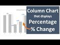
Percentage Change in Excel Charts with Color Bars - Part 2
This video is a followup to last week's video on creating a column that displays the percentage change. This iteration has colored error bars to show the positive variances in green and the negative variances in red.
Download the Excel file:
https://www.excelcampus.com/charts/column-chart-percentage-change/
The chart is also more dynamic in that it automatically displays the data labels and error bars in the correct position as the data changes. This adds conditional formatting to our chart.
I added a slicer and link the chart's source data to a pivot table using the GETPIVOTDATA function to make the chart fully interactive.
These changes were inspired by questions from Conor and Wayne on last week's video (https://youtu.be/SRTwzaTRfCc).
Thank you for the feedback!
**Excel 2010 & Earlier**
If you are using Excel 2010 or earlier you will not have the Value from Cells option for the data labels. However, you can use the free XY Labeler add-in from AppsPro to create the labels. This will save you a lot of time. Here is the link to download the add-in.
http://www.appspro.com/Utilities/ChartLabeler.htm
Related articles & videos:
Part 1: https://youtu.be/SRTwzaTRfCc
Part 3: https://youtu.be/X0ySDc5KwsM
Variance on Clustered Column for Actual versus Budget: https://www.excelcampus.com/charts/variance-clustered-column-bar-chart/
3-part Video Series on Pivot Tables & Dashboards: https://youtu.be/9NUjHBNWe9M
Free Chart Alignment Add-in: https://www.excelcampus.com/keyboard-shortcuts/chart-alignment-add-in/
Видео Percentage Change in Excel Charts with Color Bars - Part 2 канала Excel Campus - Jon
Показать
Комментарии отсутствуют
Информация о видео
Другие видео канала
 Column Chart That Displays Percentage Change in Excel - Part 1
 Dynamic Variance Arrows Chart with Check Boxes
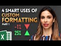 4 SMART Ways to use Custom Formatting instead of Conditional Formatting in Excel - Part 1
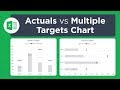 Actual vs Targets Chart in Excel
 This Excel Chart will grab your attention (Infographic template included)
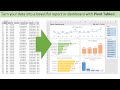 Introduction to Pivot Tables, Charts, and Dashboards in Excel (Part 1)
 Beautiful 3D Visualization in Excel
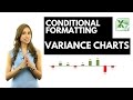 Excel Variance Charts: Actual to Previous Year or Budget Comparisons
 Secrets to Building Excel Dashboards in Under 15 Minutes!
 How to calculate the percentage change in Excel
 Better Excel Variance Charts to show percentage change (Simple & uncommon technique)
 10 Advanced Excel Charts
 Column Chart That Displays Percentage Change - Part 3
 How To Import & Clean Messy Accounting Data in Excel | Use Power Query to Import SAP Data
 Excel Magic Trick # 267: Percentage Change Formula & Chart
 Info-graphics: 3D Glass Chart in Excel
 Excel Dashboard - Plan vs Actual Variances - FREE Download
 Comparison Dashboard - Super Easy and Very Useful
 Simple Excel Trick to Conditionally Format Your Bar Charts