How to do a 2-way Lookup in Excel - Advanced MATCH and VLOOKUP Tutorial
A quick and easy tutorial on how to perform a 2-way lookup in Excel. Download the file used in this video and see more tips at http://software-matters.co.uk/microsoft-excel-help-and-tips.html#download. A 2-way lookup uses 2 pieces of lookup information to identify a piece of data, and can be done in Excel using the MATCH and VLOOKUP functions.
See more tips:
http://www.software-matters.co.uk/youtube_links.html
Music:
George Street Shuffle - Kevin MacLeod
http://incompetech.com/
----------
Visit the Software-Matters website:
http://www.software-matters.co.uk/
Software-Matters is based in Gillingham, Dorset, in the south-west of the United Kingdom (UK), near Somerset, Wiltshire and Hampshire and the cities of Bournemouth, Poole, Southampton, Bristol, Bath and Salisbury.
----------
ABRIDGED TRANSCRIPT
A 2 way lookup is required when the piece of information you need to look up requires two pieces of information to uniquely identify it. Let's look at an example. I'm creating a list in Excel of orders on a line of a piece of clothing. There are several different styles available for the item, and several different sizes. The cost to produce the item depends on both. I have arranged these costs in a small array here, and want to be able to make these costs feed into my Line costs in the orders list by getting the right amount for the style and size I specify.
I can't just lookup the style name, as I wouldn't know which column to return the price from. I need to simultaneously lookup the column number that contains the correct size, then feed that number into a VLOOKUP to get my cost.
We can use [MATCH] here to look up the column number that contains the size we want, then let our vlookup read this number. First we'll give names to the two ranges of data we'll need. First is the regular VLOOKUP data, remembering that the thing we need to lookup, the style name, should be the first column of our range. Second is the row with the size information. This second range MUST have the same width as the first and be exactly aligned above it, otherwise the 3rd column of our second range won't also be the 3rd column in our main range, for example.
Now it will be neatest if we just write the MATCH formula straight into the column argument of the vlookup, so I'll start the VLOOKUP in my Line Cost column. I'm looking up the style, in my main data range, so that deals with the first two arguments. Now for the column number I start a MATCH function, looking up the Size in the second range I specified. I enter 0 as the last argument, which makes it return only exact matches, which logically I should be able to find here.
Finally I enter false as the final argument, because I also only want exact matches on my style name. Now I just multiply the price it will be returning by the quantity of orders and I'm done! I can copy my formula down and immediately see the line costs of all my orders.
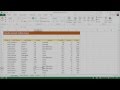
So in principle, that's all there is to it. Now we'll look at a more substantial example: I have two tables with budgeted and actual costs associated with a variety of projects for each month in a year. I'm going to use the 2-way lookup technique to create a report to compare budgets and expenses in a dynamic and automatic way.
First I need to name two ranges with the actual data in it. Then I name another range which is just the row with the month titles. Note I only need to do this once as the month rows on each table are horizontally aligned, so the column number you'll look up using MATCH will be the same in either one.
Now for each column in my report I need to know what month it should get data from. That means I need to have the title of the month above both my budget and actual column, which doesn't look all that good, so instead I have a regular title merged across all three of the columns for a month, then use another row below it with the individual month titles that I can hide later on.
So now I can start to set up my 2-way lookup formulae just as I did before. I'm looking up the name of the project in the budget data range. Next I match the month title in the row I'll hide to the month row I named.
Note that this time I put a dollar sign in front of the row number to make this an absolute reference to this row; this means all rows of my report when I copy my formula down will look at this same row to get the month name. I leave the column letter as a relative references, as I want that to change as I copy my formulae into the budget columns of other months.
Again, both the MATCH and VLOOKUP functions want to be set to use exact matches.
The variance is just the budget - the actual, so that's easy. Now I have the formulae set up for one month, I can just copy them across the whole year. The reference to the month title above the column will automatically change since it was a relative reference, so all the formulae will correct themselves to use the right months, and we're done!
Видео How to do a 2-way Lookup in Excel - Advanced MATCH and VLOOKUP Tutorial канала Software-Matters
See more tips:
http://www.software-matters.co.uk/youtube_links.html
Music:
George Street Shuffle - Kevin MacLeod
http://incompetech.com/
----------
Visit the Software-Matters website:
http://www.software-matters.co.uk/
Software-Matters is based in Gillingham, Dorset, in the south-west of the United Kingdom (UK), near Somerset, Wiltshire and Hampshire and the cities of Bournemouth, Poole, Southampton, Bristol, Bath and Salisbury.
----------
ABRIDGED TRANSCRIPT
A 2 way lookup is required when the piece of information you need to look up requires two pieces of information to uniquely identify it. Let's look at an example. I'm creating a list in Excel of orders on a line of a piece of clothing. There are several different styles available for the item, and several different sizes. The cost to produce the item depends on both. I have arranged these costs in a small array here, and want to be able to make these costs feed into my Line costs in the orders list by getting the right amount for the style and size I specify.
I can't just lookup the style name, as I wouldn't know which column to return the price from. I need to simultaneously lookup the column number that contains the correct size, then feed that number into a VLOOKUP to get my cost.
We can use [MATCH] here to look up the column number that contains the size we want, then let our vlookup read this number. First we'll give names to the two ranges of data we'll need. First is the regular VLOOKUP data, remembering that the thing we need to lookup, the style name, should be the first column of our range. Second is the row with the size information. This second range MUST have the same width as the first and be exactly aligned above it, otherwise the 3rd column of our second range won't also be the 3rd column in our main range, for example.
Now it will be neatest if we just write the MATCH formula straight into the column argument of the vlookup, so I'll start the VLOOKUP in my Line Cost column. I'm looking up the style, in my main data range, so that deals with the first two arguments. Now for the column number I start a MATCH function, looking up the Size in the second range I specified. I enter 0 as the last argument, which makes it return only exact matches, which logically I should be able to find here.
Finally I enter false as the final argument, because I also only want exact matches on my style name. Now I just multiply the price it will be returning by the quantity of orders and I'm done! I can copy my formula down and immediately see the line costs of all my orders.
So in principle, that's all there is to it. Now we'll look at a more substantial example: I have two tables with budgeted and actual costs associated with a variety of projects for each month in a year. I'm going to use the 2-way lookup technique to create a report to compare budgets and expenses in a dynamic and automatic way.
First I need to name two ranges with the actual data in it. Then I name another range which is just the row with the month titles. Note I only need to do this once as the month rows on each table are horizontally aligned, so the column number you'll look up using MATCH will be the same in either one.
Now for each column in my report I need to know what month it should get data from. That means I need to have the title of the month above both my budget and actual column, which doesn't look all that good, so instead I have a regular title merged across all three of the columns for a month, then use another row below it with the individual month titles that I can hide later on.
So now I can start to set up my 2-way lookup formulae just as I did before. I'm looking up the name of the project in the budget data range. Next I match the month title in the row I'll hide to the month row I named.
Note that this time I put a dollar sign in front of the row number to make this an absolute reference to this row; this means all rows of my report when I copy my formula down will look at this same row to get the month name. I leave the column letter as a relative references, as I want that to change as I copy my formulae into the budget columns of other months.
Again, both the MATCH and VLOOKUP functions want to be set to use exact matches.
The variance is just the budget - the actual, so that's easy. Now I have the formulae set up for one month, I can just copy them across the whole year. The reference to the month title above the column will automatically change since it was a relative reference, so all the formulae will correct themselves to use the right months, and we're done!
Видео How to do a 2-way Lookup in Excel - Advanced MATCH and VLOOKUP Tutorial канала Software-Matters
Показать
Комментарии отсутствуют
Информация о видео
Другие видео канала
 How to Extract Data from a Spreadsheet using VLOOKUP, MATCH and INDEX
 How to Perform Multiple Item Lookups in Excel (with VLOOKUP)
 How and When to use Histograms in Microsoft Excel - Tutorial with Free Download
 Excel Magic Trick 781: Three Way Lookup: INDEX and MATCH and Concatenated Ranges & Cells
 Page Layout using Adobe InDesign for Educators
 Using SUMIF in Excel - Top 5 Excel Features #2 - NO MUSIC Version
 Chattels Management Access Database - Sherborne Castle Case Study (Database Example)
 How to make Pie Charts - Microsoft Excel Tutorial
 Advanced Excel - VLOOKUP Basics
 Compare Multiple Lists with a Pivot Table
 Excel 2016 - VLOOKUP Excel 2016 Tutorial - How To Use and Do VLookup Formula Function in Office 365
 Automating Formula changes with Excel Tables - NO MUSIC Version
 Advanced Excel Index Match (3 Most Effective Formulas for Multiple Criteria)
 How to Create a Stock Management Database in Microsoft Access - Full Tutorial with Free Download
 Excel Lookup With Multiple Criteria
 How to Create Many-to-Many Relationships in Microsoft Access - Full Tutorial with Free Download
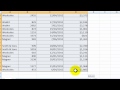 How to Delete Blank Rows in Excel
 When a Vlookup isn't working in Excel
 Excel Magic Trick 778: INDEX & MATCH Lookup Functions Beginning To Advanced (18 Examples)
 Use a VLOOKUP to Get Values for Multiple Columns