- Популярные видео
- Авто
- Видео-блоги
- ДТП, аварии
- Для маленьких
- Еда, напитки
- Животные
- Закон и право
- Знаменитости
- Игры
- Искусство
- Комедии
- Красота, мода
- Кулинария, рецепты
- Люди
- Мото
- Музыка
- Мультфильмы
- Наука, технологии
- Новости
- Образование
- Политика
- Праздники
- Приколы
- Природа
- Происшествия
- Путешествия
- Развлечения
- Ржач
- Семья
- Сериалы
- Спорт
- Стиль жизни
- ТВ передачи
- Танцы
- Технологии
- Товары
- Ужасы
- Фильмы
- Шоу-бизнес
- Юмор
PCA Explained with Python (Dimensionality Reduction Made Simple) | CodeVisium #MachineLearning
Principal Component Analysis (PCA) is one of the most widely used dimensionality reduction techniques in machine learning and data science.
It helps when datasets have:
Too many features
Correlated variables
High computational cost
Visualization challenges
PCA transforms the data into a smaller set of meaningful components while preserving the most important information.
🧠 1️⃣ What problem does PCA solve?
Many datasets contain dozens or hundreds of features.
Problems with high dimensional data:
• Slower model training
• Risk of overfitting
• Hard to visualize
• High computational cost
PCA solves this by transforming features into a smaller number of orthogonal components.
Example:
Dataset with 100 features → reduce to 10 components
You keep most information but reduce complexity.
📐 2️⃣ What are principal components?
Principal components are new features created from combinations of original features.
Properties:
• Components are uncorrelated
• Each component captures maximum variance
• First component captures the most information
Example:
Original features:
Height
Weight
Age
PCA might create:
PC1 = 0.6*Height + 0.7*Weight
PC2 = combination capturing remaining variance
📉 3️⃣ How PCA reduces dimensionality?
Steps PCA performs:
Standardize the dataset
Compute covariance matrix
Calculate eigenvectors and eigenvalues
Rank components by explained variance
Select top components
Result:
Original data → projected onto fewer dimensions.
🧮 4️⃣ Why variance is important in PCA?
Variance represents information spread.
Higher variance → more information.
PCA keeps components with highest variance because they capture the most important structure in the data.
Example:
If PC1 explains 70% variance
and PC2 explains 20%
Then two components already capture 90% of the information.
🧑💻 5️⃣ Python implementation of PCA
Using Scikit-learn:
from sklearn.decomposition import PCA
from sklearn.preprocessing import StandardScaler
from sklearn.datasets import load_iris
# Load dataset
data = load_iris()
X = data.data
# Standardize data
scaler = StandardScaler()
X_scaled = scaler.fit_transform(X)
# Apply PCA
pca = PCA(n_components=2)
X_pca = pca.fit_transform(X_scaled)
print("Explained variance:", pca.explained_variance_ratio_)
This reduces the dataset from 4 features → 2 components.
📊 Visualizing PCA
import matplotlib.pyplot as plt
plt.scatter(X_pca[:,0], X_pca[:,1])
plt.xlabel("Principal Component 1")
plt.ylabel("Principal Component 2")
plt.title("PCA Visualization")
plt.show()
This helps visualize high-dimensional data in 2D space.
🛠️ Tools commonly used for PCA
• Scikit-learn
• NumPy
• Pandas
• Matplotlib / Seaborn
• TensorFlow / PyTorch preprocessing
Used in:
Computer vision
NLP embeddings
Feature engineering
Data compression
Visualization
🎤 INTERVIEW QUESTIONS & ANSWERS
Q1. What is PCA used for?
Answer:
PCA is used for dimensionality reduction while preserving maximum variance.
Q2. What are principal components?
Answer:
Linear combinations of original features capturing maximum variance.
Q3. Why should data be standardized before PCA?
Answer:
Because PCA is sensitive to feature scale.
Q4. What do eigenvectors represent in PCA?
Answer:
Directions of maximum variance.
Q5. What do eigenvalues represent?
Answer:
Amount of variance explained by each component.
Видео PCA Explained with Python (Dimensionality Reduction Made Simple) | CodeVisium #MachineLearning канала CodeVisium
It helps when datasets have:
Too many features
Correlated variables
High computational cost
Visualization challenges
PCA transforms the data into a smaller set of meaningful components while preserving the most important information.
🧠 1️⃣ What problem does PCA solve?
Many datasets contain dozens or hundreds of features.
Problems with high dimensional data:
• Slower model training
• Risk of overfitting
• Hard to visualize
• High computational cost
PCA solves this by transforming features into a smaller number of orthogonal components.
Example:
Dataset with 100 features → reduce to 10 components
You keep most information but reduce complexity.
📐 2️⃣ What are principal components?
Principal components are new features created from combinations of original features.
Properties:
• Components are uncorrelated
• Each component captures maximum variance
• First component captures the most information
Example:
Original features:
Height
Weight
Age
PCA might create:
PC1 = 0.6*Height + 0.7*Weight
PC2 = combination capturing remaining variance
📉 3️⃣ How PCA reduces dimensionality?
Steps PCA performs:
Standardize the dataset
Compute covariance matrix
Calculate eigenvectors and eigenvalues
Rank components by explained variance
Select top components
Result:
Original data → projected onto fewer dimensions.
🧮 4️⃣ Why variance is important in PCA?
Variance represents information spread.
Higher variance → more information.
PCA keeps components with highest variance because they capture the most important structure in the data.
Example:
If PC1 explains 70% variance
and PC2 explains 20%
Then two components already capture 90% of the information.
🧑💻 5️⃣ Python implementation of PCA
Using Scikit-learn:
from sklearn.decomposition import PCA
from sklearn.preprocessing import StandardScaler
from sklearn.datasets import load_iris
# Load dataset
data = load_iris()
X = data.data
# Standardize data
scaler = StandardScaler()
X_scaled = scaler.fit_transform(X)
# Apply PCA
pca = PCA(n_components=2)
X_pca = pca.fit_transform(X_scaled)
print("Explained variance:", pca.explained_variance_ratio_)
This reduces the dataset from 4 features → 2 components.
📊 Visualizing PCA
import matplotlib.pyplot as plt
plt.scatter(X_pca[:,0], X_pca[:,1])
plt.xlabel("Principal Component 1")
plt.ylabel("Principal Component 2")
plt.title("PCA Visualization")
plt.show()
This helps visualize high-dimensional data in 2D space.
🛠️ Tools commonly used for PCA
• Scikit-learn
• NumPy
• Pandas
• Matplotlib / Seaborn
• TensorFlow / PyTorch preprocessing
Used in:
Computer vision
NLP embeddings
Feature engineering
Data compression
Visualization
🎤 INTERVIEW QUESTIONS & ANSWERS
Q1. What is PCA used for?
Answer:
PCA is used for dimensionality reduction while preserving maximum variance.
Q2. What are principal components?
Answer:
Linear combinations of original features capturing maximum variance.
Q3. Why should data be standardized before PCA?
Answer:
Because PCA is sensitive to feature scale.
Q4. What do eigenvectors represent in PCA?
Answer:
Directions of maximum variance.
Q5. What do eigenvalues represent?
Answer:
Amount of variance explained by each component.
Видео PCA Explained with Python (Dimensionality Reduction Made Simple) | CodeVisium #MachineLearning канала CodeVisium
principal component analysis pca explained dimensionality reduction python machine learning preprocessing sklearn pca tutorial data science techniques feature engineering methods eigenvectors eigenvalues pca ml interview questions ai data preprocessing python pca example data visualization ml machine learning fundamentals codevisium
Комментарии отсутствуют
Информация о видео
8 марта 2026 г. 16:23:28
00:00:10
Другие видео канала