How to Add a Search Box to a Slicer in Excel
Learn how to add a search box to a slicer to quickly filter pivot tables, pivot charts, or Excel Tables.
Click here to download the files: http://www.excelcampus.com/pivot-tables/add-search-box-to-slicer/
Here are basic instructions from the video.
The blog post page contains more screenshots and keyboard shortcuts for the filter search boxes.
http://www.excelcampus.com/pivot-tables/add-search-box-to-slicer/
1. Insert a slicer on the worksheet.
2. Make a copy of the pivot table and paste it next to the existing pivot table.
3. The new pivot table will also be connected to the slicer. The slicer is connected to both pivot tables.
4. Remove all fields from the areas of the new pivot table.
5. Add the slicer field to the Filters area of the new pivot table.
6. Move the slicer on top of the cell that contains the filter drop-down button in the Filters area of the new pivot table.
7. Adjust the column width so the filter button is just to the right of the slicer.
8. Turn off the Autofit column widths option on the new pivot table. (Right-click pivot table, PivotTable Options…)
9. Hide the column that contains the field name in the Filters area of the new pivot table.
Please subscribe to my free email newsletter to get more Excel tips like this. http://www.excelcampus.com/newsletter
Видео How to Add a Search Box to a Slicer in Excel канала Excel Campus - Jon
Показать
Комментарии отсутствуют
Информация о видео
Другие видео канала
 Custom Style for Slicers in Excel
 Using slicers with formulas in Excel | Allow users to select parameters | Excel Off The Grid
 Searchable Drop Down List in Excel (Very Easy with FILTER Function)
 Don't Use Excel Filters! Use This Incredible Excel Formula Instead ...
 Secrets to Building Excel Dashboards in Under 15 Minutes!
 Setup a Slicer to Sort or Filter Another Slicer for Quick Navigation
 Create Multiple Pivot Table Reports with Show Report Filter Pages
 Pivot Table with Progress Chart and Dashboard
 How to creat SEARCH BOX in excel sheet
 Excel Pivot Chart with Slicers for Months to Show Values by Weekday Names
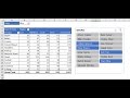 PivotTables & Slicers Made Easy! 4 Amazing Examples for WAAT Accounting Seminar August 26, 2016
 Force Excel Slicers to Single Select Using These Crafty Tricks
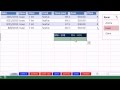 Excel Magic Trick 1056: Excel 2013 Slicer Formulas
 Create Multiple Dependent Drop-Down Lists in Excel (on Every Row)
 Dynamic Filter in Excel - Filter As You Type (with & without VBA)
 Build Impressive Charts: It's NOT your usual Bar Chart (Infographics in Excel)
![Real-Time Data Search Box in Excel with FILTER function [Part 1]](https://i.ytimg.com/vi/gHXalY5rngI/default.jpg) Real-Time Data Search Box in Excel with FILTER function [Part 1]
Real-Time Data Search Box in Excel with FILTER function [Part 1] 4 SMART Ways to use Custom Formatting instead of Conditional Formatting in Excel - Part 1
 VLOOKUP Tutorial for Excel - Everything You Need To Know