Shelly Cashman Excel 2019 | Module 5: SAM Project 1a #shellycashmanexcel #module5 #samproject1a
Shelly Cashman Excel 2019 | Module 5: SAM Project 1a #shellycashmanexcel #module5 #samproject1a
If you directly want to get the project from us then contact us on our Whatsapp. Link is given here,
Whatsapp Contact Link:
https://api.whatsapp.com/message/4B6NMKKBKUFYN1?autoload=1&app_absent=0
All Projects Link:
https://whatsapp.com/channel/0029VaBCB3P1t90m1bdQfM18
Whatsapp Number:
+919116641093
+918005564456
Gmail Id:
singhal.agrawal.bharati@gmail.com
1) Olivia Clausen is a product analyst for Media Hub, a website that sells audio books, movies, TV shows, and other media around the world. Olivia is tracking sales for the year and asks for your help in projecting future sales and visualizing the sales data.
The United States, Canada, and Australia worksheets have the same structure and contain similar data. Group the United States, Canada, and Australia worksheets to make changes to the three worksheets at the same time. The first change is to display today's date.
In cell H1 of the United States worksheet, enter a formula using the TODAY function to display today's date.
2) Find the text "Science fantasy" and then change it to Science fiction to use the more common term.
3) Use the month name in cell H5 to fill the range I5:O5 with the names of the remaining months in the year.
4) Olivia wants to use the cell formatting in merged cell H6 in other places in the workbook. Create and apply a cell style as follows:
a. Create a cell style named Subhead based on the formatting in merged cell H6.
b. Apply the new Subhead cell style to cell H8.
5) Olivia thinks Media Hub has a good chance of increasing the number of audio book downloads in the United States to 14,000 in December. For May, she estimates 11,432 downloads, which is the average number of monthly downloads from January to April.
Project the number of downloads in June to November by filling the series for the first projection (range H7:O7) with a linear trend.
6) Olivia also wants to know how the number of downloads would increase if customers downloaded 3% more audio books each month from June to December.
Project the number of downloads in June to December for the second projection (range H9:O9) based on a growth series using 1.03 as the step value.
7) Olivia wants to consolidate the sales data in the United States, Canada, and Australia on the All Locations worksheet.
Ungroup the worksheets, go to the All Locations worksheet, and then consolidate the data as follows:
a. In cell B6, enter a formula using the SUM function and a 3D reference to total the number of downloads of Adventure audio books in January (cell B6) in the United States, Canada, and Australia.
b. Copy the formula in cell B6 to calculate the number of downloads for the other types of books and months (ranges B7:B11 and C6:E11), pasting the formula only.
c. In cell B16, enter a formula using the SUM function and a 3D reference to total the sales of Adventure audio books in January (cell B16) in the United States, Canada, and Australia.
d. Copy the formula in cell B16 to calculate the sales for the other types of books and months (ranges B17:B21 and C16:E21), pasting the formula only.
8) Olivia wants to round the total sales values so that they are easier to remember.
a. In cell B22, add the ROUNDUP function to display the total sales for January rounded up to 0 decimal places.
b. Fill the range C22:F22 with the formula in cell B22.
9) In cell F24, Olivia wants to display the total sales from the previous year for the same period. This data is stored in another workbook. Insert the total as follows:
a. Open the file Support_EX19_5a_Sales.xlsx.
b. In cell F24 of Olivia's workbook, insert a formula using an external reference to cell F22 in the All Locations worksheet in the Support_EX19_5a_Sales.xlsx workbook.
10) Olivia wants to visualize how the sales of each type of audio book contributed to the total sales for January to April.
Create a chart as follows to illustrate this information:
a. Create a 3-D pie chart that shows how each type of book (range A16:A21) contributed to the total sales (range F16:F21).
b. Move and resize the chart so that the upper-left corner is in cell B25 and the lower-right corner is in cell F40.
11) Format the 3-D pie chart as follows to make it easier to interpret:
a. Use Total Sales as the chart title.
b. Add data labels to the chart on the Outside End of each slice.
c. Display only the Category Name and Percentage values in the data labels.
d. Change the number format of the data labels to Percentage with 1 decimal place.
e. Explode the largest slice (Mystery audio books) by 8 percent.
f. Remove the legend, which repeats information in the data labels.
12) Prepare for printing the All Locations worksheet as follows:
a. Change the top and bottom margins to 0.25".
b. Select the range A1:F41 as the print area.
c. Insert a footer that displays the Sheet Name in the center section.
Видео Shelly Cashman Excel 2019 | Module 5: SAM Project 1a #shellycashmanexcel #module5 #samproject1a автора Управление финансовыми операциями Excel
Видео Shelly Cashman Excel 2019 | Module 5: SAM Project 1a #shellycashmanexcel #module5 #samproject1a автора Управление финансовыми операциями Excel
Информация
5 декабря 2023 г. 21:42:10
00:01:27
Похожие видео


