Factor Analysis in SPSS (Principal Components Analysis) - Part 2 of 6
In this video, we look at how to run an exploratory factor analysis (principal components analysis) in SPSS (Part 2 of 6).
YouTube Channel: https://www.youtube.com/user/statisticsinstructor
Subscribe today!
Video Transcript: to Dimension Reduction. And first of all, notice that name there, dimension reduction. The key here, reduction, we're trying to reduce a certain number of variables or items to a smaller number of factors or components. And we can refer to these as dimensions, so if we have one factor that's a one dimension(al) solution, two factors is a two dimension(al) solution, and so on. Let's go ahead and select Factor. And then here we want to move all our variables over to the right. Go ahead and select Descriptives, and then we'll select Univariate descriptives, to get some univariate descriptive statistics on each of our variables. And I also want to select KMO and Bartlett's test of sphericity. Then we'll click Continue. And then next we go to Extraction and notice here, by default, the method is principal components. And that's what I had mentioned that we're going to run here today. So that's good, we want to leave that selected. But if you are looking for an alternative procedure, you can find a number of them here. Now We're just going to do principal components, which I said earlier, is the most commonly used method of analysis. OK we'll go ahead and leave these defaults, we'll have the Unrotated factor solution displayed, and then I also want to display a Scree plot, which I'll tell you about more in a few minutes. And then let's leave this Extraction default option selected. So notice that the extraction is, based on eigenvalue, where eigenvalues greater than 1 will be retained or extracted. And I will go into that in detail in just a few moments. So go ahead and click Continue. OK Rotations, let's go ahead and look at that. Now I'll go and select Varimax, and we'll see what happens when we run the analysis. But notice here we have five different options. The first thing to note is that there's two key types of rotation, there's Orthogonal rotation, and there's Oblique rotation. Now orthogonal rotation means that your factors or components, if there is more than one, if there's two or more factors or components, they will be uncorrelated. In fact that rotational solution forces them to be uncorrelated. Now oblique, on the other hand, they're rotated in such a way where they're allowed to be correlated. So you'll get solutions where the factors typically will be correlated to some degree. But the oblique rotation allows for the correlation. Now of these rotation procedures in SPSS, Varimax, Quartimax and Equamax are all different types of orthogonal, or uncorrelated rotations, whereas Direct Oblimin and Promax are oblique, or correlated rotations. We'll go and select Varimax in this case. OK go ahead and click Continue. And then that looks good, so go ahead and click OK. And then here we have our analysis, and our first table we'll look at here is the KMO and Bartlett's test. This is sometimes reported, so I want to be sure that you understand what it is here. Bartlett's test the sphericity, that's what we're going to be focusing on. And Bartlett's test of sphericity, notice first of all, that it is significant, it's less than .05. And it approximates a chi-square distribution, so we can consider it chi-square distributed. And what this is testing is, it's actually testing whether this correlation matrix, are these variables, so item 1 with 2, item 1 with 3, item 2 with 3, and so on, this entire triangle are these variables, are they correlated significantly different than zero. But unlike the correlation matrix, it doesn't test each individual correlation separately, but what it does is, in one overall test, it assesses whether these 10 correlations, taken as a group, do they significantly differ from zero. And more precisely, for those who are familiar with matrix algebra, it's testing whether this correlation matrix is significantly different than an identity matrix. An identity matrix just has ones along the main diagonal and zeros in all other places. So in other words, it's a matrix where variables are not correlated whatsoever with each other, but as always, a variable correlates 1.0 with itself. So it has 1s on the main diagonal, 0 everywhere else. And the fact that this is significant, and it's extremely significant, the p-value is very small, it gives us confidence that our variables are significantly correlated. So once again that's testing whether the variables, as a set, does this matrix, does this group of variables, differ significantly from all zeros here, and it definitely does. So that's what that test measures. OK next we have our commonalities, and I'm going to skip over that for a minute, we'll get back to that soon though. Let's go and look at the total variance explained.
Видео Factor Analysis in SPSS (Principal Components Analysis) - Part 2 of 6 канала Quantitative Specialists
Показать
Комментарии отсутствуют
Информация о видео
16 декабря 2014 г. 5:55:38
00:05:35
Другие видео канала
 Factor Analysis in SPSS (Principal Components Analysis) - Part 3 of 6
 Factor Analysis in SPSS (Principal Components Analysis) - Part 1
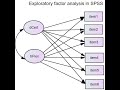 Exploratory factor analysis in SPSS (October, 2019)
 Multiple Linear Regression in SPSS with Assumption Testing
 SPSS: How to analyze and interpret Likert-Scale Questionnaire using SPSS
 SPSS #24 - KMO & Bartlett's Test of Sphericity - Factor Analysis
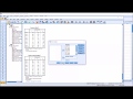 Interpreting SPSS Output for Factor Analysis
 Exploratory Factor Analysis (EFA): Concept, Key Terminologies, Assumptions, Running, Interpreting
 Factor Analysis - Factor Loading, Factor Scoring & Factor Rotation (Research & Statistics)
 Mann-Whitney U Test and Alternative Non-Parametric Tests in SPSS
 Quantitative Methoden - Fragebogen: Codierung und Datenprüfung
 Die Explorative Faktorenanalyse mit SPSS zur Analyse von Fragebögen
 Applied Principal Component Analysis in R
 Multiple Regression in SPSS - R Square; P-Value; ANOVA F; Beta (Part 1 of 3)
 Confirmatory factor analysis in AMOS (Sept 2020)
 Factor Analysis Using SPSS | Scree Plot and Total Variance Explained Table: Part 4
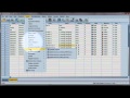 Reliability test: Compute Cronbach's alpha using SPSS
 SPSS (9): Mean Comparison Tests | T-tests, ANOVA & Post-Hoc tests
 Normality Tests in SPSS