- Популярные видео
- Авто
- Видео-блоги
- ДТП, аварии
- Для маленьких
- Еда, напитки
- Животные
- Закон и право
- Знаменитости
- Игры
- Искусство
- Комедии
- Красота, мода
- Кулинария, рецепты
- Люди
- Мото
- Музыка
- Мультфильмы
- Наука, технологии
- Новости
- Образование
- Политика
- Праздники
- Приколы
- Природа
- Происшествия
- Путешествия
- Развлечения
- Ржач
- Семья
- Сериалы
- Спорт
- Стиль жизни
- ТВ передачи
- Танцы
- Технологии
- Товары
- Ужасы
- Фильмы
- Шоу-бизнес
- Юмор
Google Sheets Dynamic Line Chart Trick with Dropdown (Show Where to Look)
📊 Google Sheets Dynamic Line Chart with Dropdown (Step-by-Step)
In this video, you’ll learn how to create a dynamic line chart in Google Sheets that automatically updates when you select a year from a dropdown.
📥 Free Template Included
I’ll share this Google Sheets template with you free of cost, so you can reuse it in your own projects.
https://docs.google.com/spreadsheets/d/1Ab_117fdnmnJH_Mz_A3KcOsyCmDzYy-PVtZ8sR5EAlo/copy
If you’re tired of static charts and want to highlight a specific year’s data, this Google Sheets line chart trick is for you.
I’ll show you how to:
Create a helper calculation table
Convert year headers into text using the TEXT function
Build a dynamic dropdown using Data Validation
Use XLOOKUP to pull year-specific data automatically
Design a clean, professional line chart
Highlight the selected year while keeping other years muted
Add custom data labels and clean formatting
This technique works perfectly when you have multi-year monthly data and want users to focus on one year at a time — ideal for dashboards, reports, and presentations.
No Apps Script. No add-ons.
Just pure Google Sheets formulas and smart chart formatting.
🎯 Why use this method?
✔ Fully dynamic
✔ Easy to update
✔ Dashboard-ready
✔ Beginner to intermediate friendly
👍 If you found this useful, don’t forget to like, subscribe, and share for more Google Sheets tips and dashboard tricks.
Chapters:
0:00 – Introduction
0:40 – Building a Helper Calculations Table
2:27 – Creating a Dropdown & Dynamic Column with XLOOKUP
4:05 – Creating and Formatting a Line Chart
Видео Google Sheets Dynamic Line Chart Trick with Dropdown (Show Where to Look) канала ExBiSheets
Google Sheets Google Sheets Tutorial Google Sheets Tips Dynamic Charts Google Sheets Line Chart Google Sheets XLOOKUP Google Sheets Dropdown Menu Google Sheets Helper Calculations Table Interactive Charts Google Sheets Data Visualization Google Sheets Spreadsheet Tutorial Google Sheets Formulas Google Sheets Dashboard Google Sheets Tricks Monthly Data Google Sheets Google Sheets Chart Formatting Dynamic Data Google Sheets Line Chart Tutorial
Комментарии отсутствуют
Информация о видео
28 декабря 2025 г. 15:03:51
00:06:43
Другие видео канала