Computational Fluid Dynamics Explained
For more information, visit https://www.airshaper.com
----------------------------------------------------------------------------------------
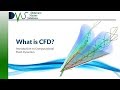
In this video, we’ll explain the basic principles of CFD or computational fluid dynamics.
Let’s start with computational: this means that in contrast to physical flows, CFD flows are simulated using computers. For simple problems, this can be done on your laptop. For bigger problems, in automotive or aviation, for example, huge clusters with thousands of cores and terabytes of memory are often used.
Secondly, it involves a fluid, which can be a liquid or a gas. When you’re working with water, it’s called hydrodynamics. When you’re working with air, it’s called aerodynamics.
Last but not least, it involves dynamics, which relates to the fluid movement.
So how does one compute a flow?
Modeling involves the continuous mathematical functions that you use to describe the real flow. In reality, that flow is the result of many different laws of physics working together. To limit computational effort, it’s a matter of selecting only the ones that have a substantial impact on your flow topic: if you’re calculating the aerodynamic force on a wing, for example, there’s little use in taking the gravitational pull of the moon into account, as the effect is negligible. So, defining correct & relevant models is important to limit the modeling errors:
In case of fluid mechanics, the most important model is a set of partial differential equations called the “Navier Stokes” equations. These basically apply the laws of Newton for every small bit of the fluid, stating the dynamic balance between the forces acting on it and the change in its momentum. This conservation of momentum, together with the conservation of mass, allows you to describe the flow field.
For some very simple cases, like laminar flow through a pipe, there are analytical solutions: the entire flow field can be described using continuous mathematical functions. These allow you to calculate the exact velocity & pressure for any given location in the flow field at an infinite resolution.
But for anything more complex than these very simple cases, we don’t have such an analytical solution. That means we need to break down reality into small blocks for which we do have a solution. These blocks can be finite elements or finite volumes, also called cells. Think of it as the difference between analog and digital photography, where a complex image is described by simple pixels, each having just one color.
This process of breaking down a large continuous flow field into small cells is called meshing. For each of these cells, we can approximate the continuous Navier-Stokes equations by discrete algebraic equations. These allow us to calculate the pressure & velocity at the center of each cell, which is called the node, based on the values of velocity & pressure of the surrounding nodes.
The higher the order of these discrete approximations, the more surrounding nodes are included. This “reach” is called the computational molecule, resulting in a set of algebraic equations for each node. As the value of one node depends on the value of neighboring nodes and vice versa, the equations are connected. This means you need to solve them simultaneously by putting them together in a big matrix.
But before we discuss how to solve this matrix, we need to talk about the discretization error: “The difference between the exact solution of the governing equations and the exact solution of the discrete approximation”. The more cells you apply, the smaller this error. But this also increases the number of equations you need to solve, and with meshes typically containing millions of cells, this quickly becomes very expensive. So you’re best off applying small cells to locations where the flow is complex, and large cells where the flow is less curvy, typically further away from the object.
Once you have defined your mesh and your matrix of equations, it’s time to solve them. It’s possible to find the exact solution of this matrix problem through a direct method like Gauss elimination or LU decomposition. But this is very costly in terms of computational power and why bother solving the equations down to computer accuracy level, when your discretization error is much bigger anyway?
This is where faster iterative methods come in: they start by “guessing” an initial solution, which could even just be a standstill flow field, or “zero velocity” for every point. Then they linearize the equations around that point and improve the solution through iteration. If you iterate long enough, the flow field will converge to a stable solution, reducing the iteration error. The difference between this solution and the direct solution of the equations is called the iteration error.
For more information, visit:
www.airshaper.com
www.facebook.com/AirShaper
www.linkedin.com/company/airshaper
#AirShaper #CFD #cfdsoftware
Видео Computational Fluid Dynamics Explained канала AirShaper
----------------------------------------------------------------------------------------
In this video, we’ll explain the basic principles of CFD or computational fluid dynamics.
Let’s start with computational: this means that in contrast to physical flows, CFD flows are simulated using computers. For simple problems, this can be done on your laptop. For bigger problems, in automotive or aviation, for example, huge clusters with thousands of cores and terabytes of memory are often used.
Secondly, it involves a fluid, which can be a liquid or a gas. When you’re working with water, it’s called hydrodynamics. When you’re working with air, it’s called aerodynamics.
Last but not least, it involves dynamics, which relates to the fluid movement.
So how does one compute a flow?
Modeling involves the continuous mathematical functions that you use to describe the real flow. In reality, that flow is the result of many different laws of physics working together. To limit computational effort, it’s a matter of selecting only the ones that have a substantial impact on your flow topic: if you’re calculating the aerodynamic force on a wing, for example, there’s little use in taking the gravitational pull of the moon into account, as the effect is negligible. So, defining correct & relevant models is important to limit the modeling errors:
In case of fluid mechanics, the most important model is a set of partial differential equations called the “Navier Stokes” equations. These basically apply the laws of Newton for every small bit of the fluid, stating the dynamic balance between the forces acting on it and the change in its momentum. This conservation of momentum, together with the conservation of mass, allows you to describe the flow field.
For some very simple cases, like laminar flow through a pipe, there are analytical solutions: the entire flow field can be described using continuous mathematical functions. These allow you to calculate the exact velocity & pressure for any given location in the flow field at an infinite resolution.
But for anything more complex than these very simple cases, we don’t have such an analytical solution. That means we need to break down reality into small blocks for which we do have a solution. These blocks can be finite elements or finite volumes, also called cells. Think of it as the difference between analog and digital photography, where a complex image is described by simple pixels, each having just one color.
This process of breaking down a large continuous flow field into small cells is called meshing. For each of these cells, we can approximate the continuous Navier-Stokes equations by discrete algebraic equations. These allow us to calculate the pressure & velocity at the center of each cell, which is called the node, based on the values of velocity & pressure of the surrounding nodes.
The higher the order of these discrete approximations, the more surrounding nodes are included. This “reach” is called the computational molecule, resulting in a set of algebraic equations for each node. As the value of one node depends on the value of neighboring nodes and vice versa, the equations are connected. This means you need to solve them simultaneously by putting them together in a big matrix.
But before we discuss how to solve this matrix, we need to talk about the discretization error: “The difference between the exact solution of the governing equations and the exact solution of the discrete approximation”. The more cells you apply, the smaller this error. But this also increases the number of equations you need to solve, and with meshes typically containing millions of cells, this quickly becomes very expensive. So you’re best off applying small cells to locations where the flow is complex, and large cells where the flow is less curvy, typically further away from the object.
Once you have defined your mesh and your matrix of equations, it’s time to solve them. It’s possible to find the exact solution of this matrix problem through a direct method like Gauss elimination or LU decomposition. But this is very costly in terms of computational power and why bother solving the equations down to computer accuracy level, when your discretization error is much bigger anyway?
This is where faster iterative methods come in: they start by “guessing” an initial solution, which could even just be a standstill flow field, or “zero velocity” for every point. Then they linearize the equations around that point and improve the solution through iteration. If you iterate long enough, the flow field will converge to a stable solution, reducing the iteration error. The difference between this solution and the direct solution of the equations is called the iteration error.
For more information, visit:
www.airshaper.com
www.facebook.com/AirShaper
www.linkedin.com/company/airshaper
#AirShaper #CFD #cfdsoftware
Видео Computational Fluid Dynamics Explained канала AirShaper
Показать
Комментарии отсутствуют
Информация о видео
Другие видео канала
 WHAT IS CFD: Introduction to Computational Fluid Dynamics
 Understanding Laminar and Turbulent Flow
 CFD Results - How to Interpret an Aerodynamic Analysis
 What's a Tensor?
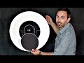 How to Understand the Black Hole Image
 Divergence and curl: The language of Maxwell's equations, fluid flow, and more
 How to become a CFD Engineer, being a Fresher? | Skill-Lync
 What is Aerodynamic Drag?
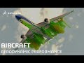 Aircraft Aerodynamic Performance | SIMULIA CFD Simulation Software
 GUTS OF CFD: Navier Stokes Equations
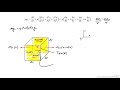 Description and Derivation of the Navier-Stokes Equations
 Sporty's Tip: Aerodynamics of a Stall
 How to run an Aerodynamic Simulation
 Why Laminar Flow is AWESOME - Smarter Every Day 208
 Design or CFD, which domain should I prefer? | Skill-Lync
 Computational Fluid Dynamic Basics
 Machine Learning for Fluid Dynamics: Patterns
 Computational Fluid Dynamics Research at the Department of Aeronautics
 Flow Visualization in Fluid Dynamics - Experiments and Methods
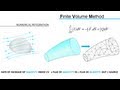 Computational Fluid Dynamics (CFD) | RANS & FVM