Lecture 5: VAR and VEC Models
This is Lecture 5 in my Econometrics course at Swansea University. Watch Live on The Economic Society Facebook page Every Monday 2:00 pm (UK time) October 2nd - December 2017.
http://facebook.com/TheEconomicSociety/
In this lecture, I explain how to estimate a vector autoregressive model. We started with explaining the Autoregressive Process to explain the behaviour of a time series and how to present such process in different forms. Then we explained the basic conditions required to estimate a VAR model. The data need to be stationary. You need to choose the optimal lag length. The model must be stable. After estimation, we could test for causality among variables using Granger causality tests. Because VAR models are often difficult to interpret, we can use the impulse responses and variance
decompositions. The impulse responses trace out the responsiveness of the dependent variables in the VAR to shocks to the error term. A unit shock is applied to each variable and its effects are noted. Variance Decomposition offers a slightly different method of examining VAR dynamics. They give the proportion of the movements in the dependent variables that are due to their ‘own’ shocks, versus shocks to the other variables. It gives information about the relative importance of each shock to the variables in the VAR.
We also covered the concept of co-integration, and how to test for cointegration. Then we discussed the Error Correction Model and Vector Error Correction Model VECM.
Видео Lecture 5: VAR and VEC Models канала Hanomics
Показать
Комментарии отсутствуют
Информация о видео
Другие видео канала
 Vector Auto Regression : Time Series Talk
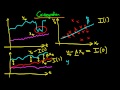 Cointegration - an introduction
 How to estimate and interpret VAR models in Eviews - Vector Autoregression model
 (EViews10): Estimate and Interpret VECM (1) #var #vecm #causality #lags #Johansen #innovations
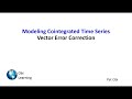 Vector Error Correction Model (VECM) - Step 4 of 4
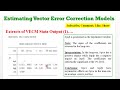 (Stata13): VECM Estimation, Discussion and Diagnostics #var #vecm #causality #granger #wald
 An Introduction to Vector Autoregressive (VAR) Models
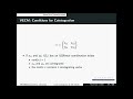 Econometrics - Vector Error Correction Model: Johansen Test
 (EViews10):Discussing Results, VAR Models(2) #var #vecm #Johansen #normality #serialcorrelation
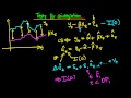 Cointegration tests
 Lecture 6: Modelling Volatility and Economic Forecasting
 Module 5: Session 12: Introduction to Structural VAR Identification
 Econometrics - Estimating VAR model in R
 Panel VECM. Model One. EVIEWS
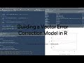 Building a Vector Error Correction Model in R
 Estimating a VAR(p) in EVIEWS
 Granger causality (prediction)
 Time Series Talk : Autoregressive Model
 (EViews10): Estimate and Interpret VECM (2) #var #vecm #causality #lags #Johansen #innovations
 Building a VAR Model in R