Understanding Wavelets, Part 2: Types of Wavelet Transforms
Explore the workings of wavelet transforms in detail.
•Try Wavelet Toolbox: https://goo.gl/m0ms9d
•Ready to Buy: https://goo.gl/sMfoDr
You will also learn important applications of using wavelet transforms with MATLAB®.
Video Transcript:
In the previous session, we discussed wavelet concepts like scaling and shifting. We will now look at two types of wavelet transforms: the Continuous Wavelet Transform and the Discrete Wavelet Transform. Key applications of the continuous wavelet analysis are: time frequency analysis, and filtering of time localized frequency components. The key application for Discrete Wavelet Analysis are denoising and compression of signals and images. As I mentioned in the previous session, these two transforms differ based on how they discretize the scale and the translation parameters. We will discuss these techniques as they apply in the 1-D scenario. Let’s take a closer look at the continuous wavelet transform – or CWT.
You can use this transform to obtain a simultaneous time frequency analysis of a signal. Analytic wavelets are best suited for time frequency analysis as these wavelets do not have negative frequency components. This list includes some analytic wavelets that are suitable for continuous wavelet analysis. The output of CWT are coefficients, which are a function of scale or frequency and time. Let’s now discuss the process of constructing different wavelet scales. Recall from our previous video that, when you scale a wavelet by a factor of 2, it results in reducing the equivalent frequency by an octave. With the CWT, you have the added flexibility to analyze the signal at intermediary scales within each octave. This allows for fine scale analysis. This parameter is referred as the number of scales per octave (Nv). The higher the number of scales per octave, the finer the scale discretization.
Typical values for this parameter are 10, 12, 16, and 32. The scales are multiplied with the sampling interval of the signal to obtain a physical significance. Here is an example of scales for a bump wavelet with 32 scales per octave. The signal is sampled every 7 micro seconds. This is the corresponding plot with the equivalent frequency for the scales. Notice that the actual scale values are exponential. Now, each scaled wavelet is shifted in time along the entire length of the signal and compared with the original signal. You can repeat this process for all the scales, resulting in coefficients that are a function of the wavelet’s scale and shift parameter. To put it in perspective, a signal with 1000 samples analyzed with 20 scales results in 20,000 coefficients.
In this way, you can better characterize oscillatory behavior in signals with the Continuous wavelet transform. The discrete wavelet transform or DWT is ideal for denoising and compressing signals and images, as it helps represent many naturally occurring signals and images with fewer coefficients. This enables a sparser representation. The base scale in DWT is set to 2. You can obtain different scales by raising this base scale to integer values represented in this way. The translation occurs at integer multiples represented in this equation. This process is often referred to as a dyadic scaling and shifting.
This kind of sampling eliminates redundancy in coefficients. The output of the transform yields the same number of coefficients as the length of the input signal. Therefore, it requires less memory. The discrete wavelet transform process is equivalent to comparing a signal with discrete multirate filter banks. Conceptually, here is how it works: Given a signal - S, - the signal is first filtered with special lowpass and high pass filter to yield lowpass and highpass sub-bands.
We can - refer to these as A1 and D1. Half of the samples are discarded after filtering as per the Nyquist criterion. The filters typically have a small number of coefficients and result in good computational performance. These filters also have the ability to reconstruct the sub bands, while cancelling any aliasing that occurs due to downsampling. For the next level of decomposition, the lowpass subband (A1) is iteratively filtered by the same technique to yield narrower subbands - A2 and D2 and so on. The length of the coefficients in each sub band is half of the number of coefficients in the preceding stage. With this technique, you can capture the signal of interest with a few large magnitude DWT coefficients, while the noise in the signal results in smaller DWT coefficients. This way, the DWT helps analyze signals at progressively narrower subbands at different resolutions. It also helps denoise and compress signals.
Видео Understanding Wavelets, Part 2: Types of Wavelet Transforms канала MATLAB
Показать
Комментарии отсутствуют
Информация о видео
Другие видео канала
 Understanding Wavelets, Part 1: What Are Wavelets
 8 1 W2 L5 P1 Introduction to Wavelets 12 40
 Wavelet Transform Based Power System Fault Detection in SIMULINK | Dr. J. A. Laghari
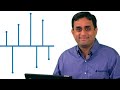 Understanding Wavelets, Part 3: An Example Application of the Discrete Wavelet Transform
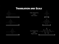 Easy Introduction to Wavelets
 Signal Analysis Made Easy
 CNN: Convolutional Neural Networks Explained - Computerphile
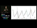 Two Effective Algorithms for Time Series Forecasting
 Partial Discharge Causes, Effects, & Online Detection Techniques 1
 The Wavelet Transform for Beginners
 Understanding Wavelets, Part 4: An Example Application of Continuous Wavelet Transform
 Wavelets and Multiresolution Analysis
 Python Scipy signal.find_peaks() -- A Helpful Guide
 What is Daubechies Wavelet? | Wavelet Theory | Advanced Digital Signal Processing
 Morlet wavelets in time and in frequency
 Wavelet transform for Images
 Wavelet Decomposition in Matlab | Wavelet Toolbox and Manual Coding
 How to inspect time-frequency results
![[Week 16-2&3] Hybrid and Switched Control Systems](https://i.ytimg.com/vi/XPQ9_NWOycM/default.jpg) [Week 16-2&3] Hybrid and Switched Control Systems
[Week 16-2&3] Hybrid and Switched Control Systems