- Популярные видео
- Авто
- Видео-блоги
- ДТП, аварии
- Для маленьких
- Еда, напитки
- Животные
- Закон и право
- Знаменитости
- Игры
- Искусство
- Комедии
- Красота, мода
- Кулинария, рецепты
- Люди
- Мото
- Музыка
- Мультфильмы
- Наука, технологии
- Новости
- Образование
- Политика
- Праздники
- Приколы
- Природа
- Происшествия
- Путешествия
- Развлечения
- Ржач
- Семья
- Сериалы
- Спорт
- Стиль жизни
- ТВ передачи
- Танцы
- Технологии
- Товары
- Ужасы
- Фильмы
- Шоу-бизнес
- Юмор
How to create a Bar Chart with Color Ranges based on Numeric Value in Excel
Do you want to automatically color bars in a chart based on data ranges? For example, values less than 60 are displayed as red bars, 60 to 69 as orange bars, 70 to 79 as blue bars and so on? This video will show you how to do this in Microsoft Excel, for both a vertical column chart and a horizontal row chart.
....................................................
PRACTICE FILE - click this link to download the Excel workbook used in the video (it will download to the default download directory on your computer):
https://datadesignstyle.com/wp-content/uploads/2025/01/Practice_ChartColorRanges_byDataDesignStyle.xlsx
....................................................
CHAPTERS:
00:00 Introduction
00:24 Define data ranges
00:38 Append columns
01:07 Write formulas
04:16 Create column chart
06:33 Sort column chart
06:50 Create row chart
07:29 Sort row chart
....................................................
Website: https://www.DataDesignStyle.com
Video is made using Filmora.
Видео How to create a Bar Chart with Color Ranges based on Numeric Value in Excel канала Data Design Style
....................................................
PRACTICE FILE - click this link to download the Excel workbook used in the video (it will download to the default download directory on your computer):
https://datadesignstyle.com/wp-content/uploads/2025/01/Practice_ChartColorRanges_byDataDesignStyle.xlsx
....................................................
CHAPTERS:
00:00 Introduction
00:24 Define data ranges
00:38 Append columns
01:07 Write formulas
04:16 Create column chart
06:33 Sort column chart
06:50 Create row chart
07:29 Sort row chart
....................................................
Website: https://www.DataDesignStyle.com
Video is made using Filmora.
Видео How to create a Bar Chart with Color Ranges based on Numeric Value in Excel канала Data Design Style
Комментарии отсутствуют
Информация о видео
24 января 2025 г. 0:33:58
00:08:10
Другие видео канала