Hopf Bifurcation Diagram with Vector Field (with audio)
With some BASS, check out
https://www.youtube.com/watch?v=EtjdjrKu9Jk
This video is a copy of http://www.youtube.com/watch?v=tTZmTbbLEps&list=TL0Xzl1jbbR6U except with the following audio explanation:
This video illustrates the formation of a hopf bifurcation for the parameter, mu. This example has two nullclines: the red curve shows no change in the x direction, and along the blue curve, there is no change in the y direction. As is with all bifurcation plots, the parameter is like a dial on a radio that we could tune while observing any fundamental changes to the vector field.
When mu is negative (as shown now), there is only 1 stable equilibrium, and it is the origin. Then when mu is greater than or equal to zero, the branch of equilibria bifurcates producing a stable limit cycle in the counter-clockwise direction. The origin has now become unstable, so trajectories near it spiral away from it and approach the circular limit cycle.
The example here is commonly used for instruction because one can change variables to polar coordinates and analyze the limit cycle in terms of its radial and angular variables without too much headache.
Видео Hopf Bifurcation Diagram with Vector Field (with audio) канала Jonathan Mitchell
Показать
Комментарии отсутствуют
Информация о видео
Другие видео канала
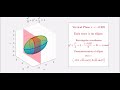 What is an Ellipsoid? (Coordinate Plane Traces)
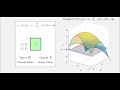 What is a Function of 2 Variables? Polynomial Example
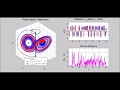 Channel Trailer - 2020
 What are Spherical Coordinates?
 What does the Tangent graph look like?
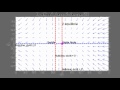 2D Transcritical Bifurcation Vector Field
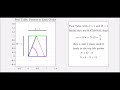 Collisions on a Square Billiards Table with Rational Slope
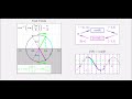 Trig Compositions: inverse cosine of cosine of theta
 Taylor Series for the Natural Exponential: f(x)=exp(x) (with audio)
 What is a Function of 2 Variables? Slanted Plane Example
 PDE Simulations: Heat Equation, Fixed BC, Low Diffusivity, Piecewise Linear IC
 PDE Simulations: Klein-Gordon Equation, Free BCs, Quadratic Nonlinearity
 Fourier Series with Complex Harmonics as Clocks - Airfoil Example
 Supplemental Vids For Diff Eq. - Sec 2.1 Phase Plane for Harmonic Osc Ex (a)
 Mass-Spring System - Undamped with Activated Periodic Forcing
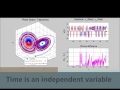 For Instructors: A 1st Look at My Channel
 What is SOH CAH TOA?
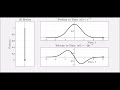 1D Motion: Position and Velocity
 1D Motion: Position, Velocity, and Acceleration
 Fundamental Theorem of Calculus (part 2) - Proof
 Lagrange Multipliers - Example 1 for MATH 5390