Double Pendulum Chaos Light Writing (computer simulation) 1

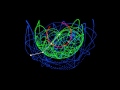
Double pendulum comprising two rigid linkages of negligible mass with point masses attached to the ends of the linkages, confined to two dimensional rotational motion about their joints without any dissipation. Here the double pendulum is held at 90 degrees and then released. Initially the motion appears regular, but chaos soon sets in, with the end point of the pendulum eventually covering the whole space available to it for a given starting energy.

The double pendulum is a wonderful example of how chaos exists in even a simple, non-dissipative, un-forced rigid 2DOF system! In this universe, chaos truly is the rule rather than the exception. In the same way as turbulent flow is well mixed, the end point of this pendulum is also "well mixed" in the sense that it has explored all of the space energetically available to it.

The linkages are coloured according to the instantaneous tension. A red colour scheme is employed during tension and a blue colour scheme during compression.

A point source of light is placed at the pendulum end point and an exposure map is created by accumulating this light on the pixels that it traverses throughout the simulation. The light source has a Gaussian spread with standard deviation of 2 pixels for added realism. So for a given point at which the light happens to be, a square grid of 4 standard deviations is placed around that point and an array is incremented at those indices with the Gaussian spread function evaluated on that square grid. An arbitrary luminosity factor scales the array before it is output as colour on a bitmap to give the desired amount of "glow". The colour values in all channels are clamped to 255 and this gives the effect of over-exposure (rather than re-scaling the intensities which would cause a dimming of everything else). This simulation of a long-time exposure photograph reveals not only where the pendulum tip has been, but also gives and indication of how fast it was going at that position and also how frequently it passed through the same path. The slower the pendulum travels, the more saturated the pixels become with the light. Also the more times the pendulum crosses the same point, the more exposed that point becomes.

All equations derived from scratch using Newtonian formulation rather than Lagrangian, by hand. You learn nothing by using symbolic maths software, and they never factorise the result in a physically meaningful way. Look at the equation at the start, notice how the masses only appear as a ratio, never alone. Thus the dynamics would be identical if both masses were scaled up or down by the same factor, i.e. if I use two 1kg masses or two 100kg masses, the end result is identical. This is because all masses fall at the same rate (Galileo). For a given set of masses, it is the length of the pendulum linkages that alter the dynamics.

All coded from scratch using Visual basic .NET. The numerical integration scheme was standard Runge-Kutta 4th order (non-symplectic, so should not be used to model long-term dynamics).

The frames of the movie were specifically output to play back in real time. So this video represents 1 minute of real time dynamics.

Pendulum parameters:
Link 1 length = 1.0m
Link 2 length = 0.9m
Mass 1 = 1.0kg
Mass 2 = 0.9kg
g = 9.81m/s^2
dt=0.0005s

The time step was ascertained by implementing a variable time step RK4 routine and observing the smallest time step ever encountered in the simulation with the tolerance on angular error specified as 1E-11 rad. For the purposes of constant frame-rate animation / movie, a constant time step must be used.

Видео Double Pendulum Chaos Light Writing (computer simulation) 1 канала Paul Nathan