KD-Tree Nearest Neighbor Data Structure
KD-Tree is a data structure useful when organizing data by several criteria all at once. Consider an example where you have a set of points on a 2 dimensional plane. Now suppose you are asked to find the nearest neighbor of some target point. What data structure would you use to store these points to be able to solve that problem?
https://en.wikipedia.org/wiki/K-d_tree
A naive approach would be to perhaps store the points in an array, sorted by one of the properties, such as the X coordinate. Then you could easily do a binary search to find the point with the closest X coordinate. But unfortunately you’d still not necessarily be any closer to finding a point where the Y coordinate is also nearby. To convince yourself of it, just think of the case where all of the points share the same X coordinate. Clearly, you’d have to examine every single point, one by one, to find the nearest neighbor of the target point.
KD-Tree data structure is much like the regular binary search tree that you are familiar with. Except each node would typically hold not just 1 value, but a list of values. When traversing a KD-Tree, we cycle through the index to the values list, based on the depth of a particular node.
The “K” in the name “KD-Tree” refers to the number of properties that each data point has. In our example, since it’s a 2 dimensional plane, we have exactly 2 properties - the X coordinate and the Y coordinate. So, the root node starts off arbitrarily picking one of those. Let’s suppose it’s the x coordinate. Then its children, the second level, alternate to using the Y coordinate. The grandchildren nodes cycle back to using the X coordinate, and so on.
Java source code:
https://bitbucket.org/StableSort/play/src/master/src/com/stablesort/kdtree/KDTree.java
When inserting a new node, just like in the typical binary search tree, we compare the node’s value and go left if it’s smaller, right if it’s bigger. It’s just that, as we go deeper and deeper down the tree, we keep alternating between using the X and the Y values in the comparison.
Note that in our example, since we started with comparing the X values, the Y values were ignored and as a consequence the 2nd layer nodes break the binary search tree rule where all nodes less than the root are on the left side and vice versa. But amazingly, it turns out that this is OK! The magic here is that we can check for this inconsistency on the way back, when unwinding the recursion.
Visually you can think of the root node dividing the XY plane into left and right sides, since we decided to start off using the X coordinate. Then the next point will fall into either the left or the right side and in turn divide that side into top and bottom sections. So as more and more nodes are inserted into the tree, each point splits the parent’s section into 2 sub-sections, alternating between splitting the section into left and right, vs top and bottom.
Once we have gone as far down as we can, we then recurse back, as you would in a regular binary tree search. We do have a candidate closest neighbor, but there is a possibility of a closer point still.
Think of the shortest distance as a line going from the target point to the candidate point. Let’s call this line “r”. This line is probably going to be at some random diagonal angle. But if the line directly perpendicular to the section that we chose not to visit when recursing down, is shorter, then there is a chance that that section may have a closer point.
So this is where the magic happens - as we recurse back, we also calculate the distance to the section that we did not visit. If that distance, let’s call it r-prime, is smaller than the best distance found so far, then we traverse into that section as well.
But note that this does not mean that we visit every node in the tree. If the height of the tree is H, then at most we’ll visit 2H nodes. In other words, this is still a logarithmic search in respect to the number of nodes in the tree.
So far we have been using an example of a 2 dimensional plane. But the methodology works equally well in higher dimensions. Each node would still just have a left and a right branch, but the number of values stored in a node could be arbitrarily large.
Suppose you are designing a database for a hospital that keeps track of each patient’s blood type, white blood cell count and blood pressure. Then a new patient comes in with an unknown illness. Using a KD-Tree you would be able to quickly select one or even a set of patients that share similar properties. These would be the “nearest neighbors”, with a higher likelihood of having a similar illness.
Видео KD-Tree Nearest Neighbor Data Structure канала Stable Sort
Показать
Комментарии отсутствуют
Информация о видео
Другие видео канала
 StatQuest: K-nearest neighbors, Clearly Explained
 K-d Trees - Computerphile
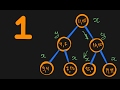 K-d Tree in Python #1 — NNS Problem and Parsing SVG
 Coding Challenge #98.1: Quadtree - Part 1
 Advanced Data Structures: K-D Trees
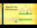 Segment Tree Data Structure - Min Max Queries - Java source code
 034 r tree
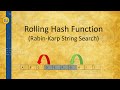 Rolling Hash Function Tutorial, used by Rabin-Karp String Searching Algorithm
 10. Introduction to Learning, Nearest Neighbors
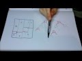 KD-Trees and Range search
 Partition to K Equal Sum Subsets - source code & running time recurrence relation
 Approximate Nearest Neighbors : Data Science Concepts
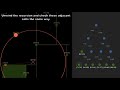 K-D Tree: build and search for the nearest neighbor
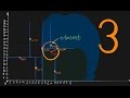 K-d Tree in Python #3 — Finale
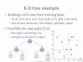 KD tree algorithm: how it works
 Building Collision Simulations: An Introduction to Computer Graphics
 10.1 AVL Tree - Insertion and Rotations
 Data Structures: Linked Lists
 Fenwick Tree (Binary Index Tree) - Quick Tutorial and Source Code Explanation
 Red-Black Trees - Data Structures