- Популярные видео
- Авто
- Видео-блоги
- ДТП, аварии
- Для маленьких
- Еда, напитки
- Животные
- Закон и право
- Знаменитости
- Игры
- Искусство
- Комедии
- Красота, мода
- Кулинария, рецепты
- Люди
- Мото
- Музыка
- Мультфильмы
- Наука, технологии
- Новости
- Образование
- Политика
- Праздники
- Приколы
- Природа
- Происшествия
- Путешествия
- Развлечения
- Ржач
- Семья
- Сериалы
- Спорт
- Стиль жизни
- ТВ передачи
- Танцы
- Технологии
- Товары
- Ужасы
- Фильмы
- Шоу-бизнес
- Юмор
Exp_19_Excel_Ch07_HOEAssessment_Employees | How to do Exp19 Excel Ch07 HOEAssessment Employees
Contact Me For Help in Your Assignments and Courses
WhatsApp : +923209088014
Email : myitlabservice@gmail.com
WhatsApp Direct Link :https://wa.me/923209088014
Tired of MYITLAB hurdles? Welcome to your digital toolbox! This channel breaks down MyITLab's features into bite-sized, practical tutorials. We'll show you how to conquer assignments, master software skills, and troubleshoot common issues. Think of us as your personal IT tutor, always ready to simplify the complex and empower you to succeed.
We can do complete MyITLab course , Microsoft Word ,Microsoft PowerPoint , Microsoft Excel , Microsoft Access.
#Exp_19_Excel_Ch07_HOEAssessment_Employees
#Exp 19 Excel Ch07 HOEAssessment Employees
#Exp19ExcelCh07HOEAssessmentEmployees
#exp_19_excel_ch07_hoeassessment_employees
#exp 19 excel ch07 hoeassessment employees
#exp19excelch07hoeassessmentemployees
#Excel_Training
#Excel Training
#Excel_training
#excel_training
#excel_Training
#exceltraining
#ExcelTraining
Steps to Perform:
Step Instructions Points Possible
1 Start Excel. Download and open the file named Exp19_Excel_Ch07_HOEAssessment_Employees.xlsx. Grader has automatically added your last name to the beginning of the filename. 0
2 The 1-Data worksheet contains employee data. You will insert several functions to complete this worksheet. Column C contains the actual hire dates for the employees. You want to extract only the year in column G.
In cell G9, insert the appropriate date function to extract the year from the date in cell C9. Copy the function from cell G9 to the range G10:G33. 3
3 Next, you want to determine how many years each employee has worked for the company.
In cell H9, insert the YEARFRAC function to calculate the years between the hire date and the last day of the year contained in cell G2. Use a mixed reference to cell G2. Copy the function from cell H9 to the range H10:H33. 3
4 You want to determine what day of the week each employee was hired.
In cell I9, insert the WEEKDAY function to display the day of the week the first employee was hired. Use 2 as the return_type. Copy the function from cell I9 to the range I10:I33. 4
5 The value returned in cell I9 is a whole number. You want to display the weekday equivalent.
In cell J9, insert a VLOOKUP function to look up the value stored in cell I9, compare it to the array in the range H2:I6, and return the day of the week. Use mixed references to the table array. Copy the function from cell J9 to the range J10:J33. 5
6 Column D contains the city each employee works in. You want to display the state.
In cell F9, insert the SWITCH function to switch the city stored in cell D9 with the respective state contained in the range C2:C4. Switch Des Moines for Iowa, St. Paul for Minnesota, and Milwaukee for Wisconsin. Use mixed references to cells C2, C3, and C4. Copy the function from cell F9 to the range F10:F33. 4
7 Your next task is to calculate the bonus for the first employee. If the employee was hired before 1/1/2010, the employee's salary is multiplied by 3%. If the employee was hired before 1/1/2015, the employee's salary is multiplied by 2%. If the employee was hired before 1/1/2020, the employee's salary is multiplied by 1%.
In cell K9, insert the IFS function to create the three logical tests to calculate the appropriate bonus. Use mixed references to cells within the range K2:L4. Copy the function from cell K9 to the range K10:K33. 5
8 Top management decided to ensure all representatives' salaries are at least $62,000 (cell G2).
In cell L9, nest an AND function within an IF function. If the job title is Representative and the salary is less than the minimum representative salary, calculate the difference between the minimum representative salary and the actual salary. If not, return zero. Use a mixed reference to cell G3. Copy the function from cell L9 to the range L10:L33. 5
9 The 2-Summary worksheet contains data to insert conditional math and statistical functions to provide summary data. First, you want to count the number of employees in each state.
Click the 2-Summary worksheet. In cell J3, insert the COUNTIF function to count the number of employees in Iowa, using the state abbreviation column and the state abbreviation in cell I3. Use mixed references for the range and cell to keep the row numbers the same. Copy the function from cell J3 to the range J4:J5. 5
10 Next, you want to calculate the total payroll for each state.
In cell K3, insert the SUMIF function to total the salaries for employees who work in Iowa, using the state abbreviation column and the state abbreviation in cell I3. Use mixed references for the ranges and cell to keep the row numbers the same. Copy the function from cell K3 to the range K4:K5.
#Exp_19_Excel_Ch07_HOEAssessment_Employees
#exp_19_excel_ch07_hoeassessment_employees
#exp19excelch07hoeassessmentemployees
#Excel_Training
#Excel Training
#Excel_training
#excel_training
#excel_Training
#exceltraining
#ExcelTraining
Видео Exp_19_Excel_Ch07_HOEAssessment_Employees | How to do Exp19 Excel Ch07 HOEAssessment Employees канала MyITLAB Service
WhatsApp : +923209088014
Email : myitlabservice@gmail.com
WhatsApp Direct Link :https://wa.me/923209088014
Tired of MYITLAB hurdles? Welcome to your digital toolbox! This channel breaks down MyITLab's features into bite-sized, practical tutorials. We'll show you how to conquer assignments, master software skills, and troubleshoot common issues. Think of us as your personal IT tutor, always ready to simplify the complex and empower you to succeed.
We can do complete MyITLab course , Microsoft Word ,Microsoft PowerPoint , Microsoft Excel , Microsoft Access.
#Exp_19_Excel_Ch07_HOEAssessment_Employees
#Exp 19 Excel Ch07 HOEAssessment Employees
#Exp19ExcelCh07HOEAssessmentEmployees
#exp_19_excel_ch07_hoeassessment_employees
#exp 19 excel ch07 hoeassessment employees
#exp19excelch07hoeassessmentemployees
#Excel_Training
#Excel Training
#Excel_training
#excel_training
#excel_Training
#exceltraining
#ExcelTraining
Steps to Perform:
Step Instructions Points Possible
1 Start Excel. Download and open the file named Exp19_Excel_Ch07_HOEAssessment_Employees.xlsx. Grader has automatically added your last name to the beginning of the filename. 0
2 The 1-Data worksheet contains employee data. You will insert several functions to complete this worksheet. Column C contains the actual hire dates for the employees. You want to extract only the year in column G.
In cell G9, insert the appropriate date function to extract the year from the date in cell C9. Copy the function from cell G9 to the range G10:G33. 3
3 Next, you want to determine how many years each employee has worked for the company.
In cell H9, insert the YEARFRAC function to calculate the years between the hire date and the last day of the year contained in cell G2. Use a mixed reference to cell G2. Copy the function from cell H9 to the range H10:H33. 3
4 You want to determine what day of the week each employee was hired.
In cell I9, insert the WEEKDAY function to display the day of the week the first employee was hired. Use 2 as the return_type. Copy the function from cell I9 to the range I10:I33. 4
5 The value returned in cell I9 is a whole number. You want to display the weekday equivalent.
In cell J9, insert a VLOOKUP function to look up the value stored in cell I9, compare it to the array in the range H2:I6, and return the day of the week. Use mixed references to the table array. Copy the function from cell J9 to the range J10:J33. 5
6 Column D contains the city each employee works in. You want to display the state.
In cell F9, insert the SWITCH function to switch the city stored in cell D9 with the respective state contained in the range C2:C4. Switch Des Moines for Iowa, St. Paul for Minnesota, and Milwaukee for Wisconsin. Use mixed references to cells C2, C3, and C4. Copy the function from cell F9 to the range F10:F33. 4
7 Your next task is to calculate the bonus for the first employee. If the employee was hired before 1/1/2010, the employee's salary is multiplied by 3%. If the employee was hired before 1/1/2015, the employee's salary is multiplied by 2%. If the employee was hired before 1/1/2020, the employee's salary is multiplied by 1%.
In cell K9, insert the IFS function to create the three logical tests to calculate the appropriate bonus. Use mixed references to cells within the range K2:L4. Copy the function from cell K9 to the range K10:K33. 5
8 Top management decided to ensure all representatives' salaries are at least $62,000 (cell G2).
In cell L9, nest an AND function within an IF function. If the job title is Representative and the salary is less than the minimum representative salary, calculate the difference between the minimum representative salary and the actual salary. If not, return zero. Use a mixed reference to cell G3. Copy the function from cell L9 to the range L10:L33. 5
9 The 2-Summary worksheet contains data to insert conditional math and statistical functions to provide summary data. First, you want to count the number of employees in each state.
Click the 2-Summary worksheet. In cell J3, insert the COUNTIF function to count the number of employees in Iowa, using the state abbreviation column and the state abbreviation in cell I3. Use mixed references for the range and cell to keep the row numbers the same. Copy the function from cell J3 to the range J4:J5. 5
10 Next, you want to calculate the total payroll for each state.
In cell K3, insert the SUMIF function to total the salaries for employees who work in Iowa, using the state abbreviation column and the state abbreviation in cell I3. Use mixed references for the ranges and cell to keep the row numbers the same. Copy the function from cell K3 to the range K4:K5.
#Exp_19_Excel_Ch07_HOEAssessment_Employees
#exp_19_excel_ch07_hoeassessment_employees
#exp19excelch07hoeassessmentemployees
#Excel_Training
#Excel Training
#Excel_training
#excel_training
#excel_Training
#exceltraining
#ExcelTraining
Видео Exp_19_Excel_Ch07_HOEAssessment_Employees | How to do Exp19 Excel Ch07 HOEAssessment Employees канала MyITLAB Service
#Exp_19_Excel_Ch07_HOEAssessment_Employees #Exp 19 Excel Ch07 HOEAssessment Employees #Exp19ExcelCh07HOEAssessmentEmployees #exp_19_excel_ch07_hoeassessment_employees #exp 19 excel ch07 hoeassessment employees #exp19excelch07hoeassessmentemployees #Excel_Training #Excel Training #Excel_training #excel_training #excel_Training #exceltraining #ExcelTraining
Комментарии отсутствуют
Информация о видео
28 марта 2025 г. 7:18:10
00:23:23
Другие видео канала